Poster

After working all night I finally finished the slide for the EUReKA conference. Here it is....

KNN Distance Metric Comparisons

I just finished running a comparison of K-nearest neighbor using euclidean distance and chi-squared (I've been using euclidean this whole time). And what do you know, using chi-squared distance got me consistently better results. Here's the results of the tests:

KNN (k=3)

Night Images:

Euclidean Distance:

1. 92% accuracy, # test images = 41
2. 85% accuracy, # test images = 41
3. 87% accuracy, # test images = 41
4. 85% accuracy, # test images = 41
5. 90% accuracy, # test images = 41

Chi-Squared Distance:

1. 92% accuracy, # test images = 41
2. 90% accuracy, # test images = 41
3. 90% accuracy, # test images = 41
4. 90% accuracy, # test images = 41
5. 95% accuracy, # test images = 41

Day Images:

Euclidean Distance:

1. 75% accuracy, # test images = 41
2. 76% accuracy, # test images = 41
3. 81% accuracy, # test images = 41
4. 76% accuracy, # test images = 41
5. 84% accuracy, # test images = 41

Chi-Squared Distance:

1. 77% accuracy, # test images = 41
2. 84% accuracy, # test images = 41
3. 85% accuracy, # test images = 41
4. 78% accuracy, # test images = 41
5. 85% accuracy, # test images = 41

Here are some visual examples of the differences in the results from Chi-Squared and Euclidean Distances:

Chi-Square 1

Euclidean 1

Chi-Square 2

Euclidean 2

Chi-Square 3

Euclidean 3

Viewing Night Results

Photobucket Album

Green = empty space, White = occupied space, Blue = Misclassified Space

So I just finished writing a combination of programs which gather up the results from the k-fold validation testing and visualizes these results (ie creates a set of result pictures). You can go to my photo bucket account and view the results from the night set.

Night and Day

I have been gathering more training data and the increase from 650 total images to 740 has made a visible difference in the detection rates for the KNN classifier.

I have been experimenting with the idea of splitting the image set into smaller sets related to the time of day and general lighting level. Other than the benefits of reducing the KNN classification time, these time-specific images sets noticeably increase the detection rates. The following is results of my tests so far:

KNN (K=3)

All Images:

1. 79% accuracy, # test images = 148
2. 80% accuracy, # test images = 147
3. 84% accuracy, # test images = 148
4. 78% accuracy, # test images = 148
5. 78% accuracy, # test images = 149

Day Images:

1. 80% accuracy, # test images = 107
2. 83% accuracy, # test images = 107
3. 66% accuracy, # test images = 106
4. 82% accuracy, # test images = 107
5. 78% accuracy, # test images = 109

Night Images:

1. 90% accuracy, # test images = 41
2. 90% accuracy, # test images = 41
3. 90% accuracy, # test images = 41
4. 82% accuracy, # test images = 41
5. 80% accuracy, # test images = 41

SVM

All Images:

1. 78% accuracy, # test images = 148
2. 76% accuracy, # test images = 147
3. 78% accuracy, # test images = 148
4. 68% accuracy, # test images = 148
5. 76% accuracy, # test images = 149

Day Images:

1. 75% accuracy, # test images = 107
2. 76% accuracy, # test images = 107
3. 59% accuracy, # test images = 106
4. 75% accuracy, # test images = 107
5. 66% accuracy, # test images = 109

Night Images:

1. 70% accuracy, # test images = 41
2. 85% accuracy, # test images = 41
3. 68% accuracy, # test images = 41
4. 75% accuracy, # test images = 41
5. 63% accuracy, # test images = 41

KNN > SVM

I just finished fixing my K-nearest neighbor program and what do you know, its detection rate is consistently better than the svm. The results on the k-fold cross-validation testing where k=5 is:

KNN

(K=1)

1. 72% accuracy, # test images = 129
2. 82% accuracy, # test images = 129
3. 75% accuracy, # test images = 129
4. 74% accuracy, # test images = 128
5. 77% accuracy, # test images = 129

(K=3)

1. 79% accuracy, # test images = 129
2. 83% accuracy, # test images = 129
3. 77% accuracy, # test images = 129
4. 75% accuracy, # test images = 128
5. 77% accuracy, # test images = 129

(K=5)

1. 75% accuracy, # test images = 129
2. 86% accuracy, # test images = 129
3. 81% accuracy, # test images = 129
4. 73% accuracy, # test images = 128
5. 77% accuracy, # test images = 129

(K=7)

1. 79% accuracy, # test images = 129
2. 84% accuracy, # test images = 129
3. 76% accuracy, # test images = 129
4. 74% accuracy, # test images = 128
5. 79% accuracy, # test images = 129

SVM

1. 79% accuracy, # test images = 129
2. 65% accuracy, # test images = 129
3. 59% accuracy, # test images = 129
4. 62% accuracy, # test images = 128
5. 71% accuracy, # test images = 129

Personally, I find these results very interesting....

Cross-validation and KNN

Throughout the week I have been taking pictures of parking lots as I have walked to and from school each day. However, the number of ROI from my image set is still pretty small, around 650 distinct parking spaces, and this may be adversely affecting my training efforts. Most research papers that I've read have said that good results are often achieved with somewhere between 1000 and 2000 bits of training data.

The next thing that I did was to implement a cross-validation script. I ended up coding a K-fold in python which starts by randomizing the input data and then performs the cross validation. With K=5, the svm is classifying within a range of 59%-79% positive detection rate. This extremely wide range might be the result of poor randomization of the data on the part of the script and/or it might be due to the fact that I have very few night time images as part of my test data. Right now I'm going to increase the size of my test set and see if that has an effect in reducing the range of results returned by the cross-validation script.

The last thing that I worked on was to create a K-nearest neighbor classification program. I am still trying to debug the program but I hope to have it done sometime tonight or tomorrow.

SVMs

So I installed, trained, and ran SVMLight today. I used some images which weren't part of the training set and which were taken on completely different days than those taken for the training set (ie, no obviously similar images being used to train and test at the same time). However, these images were quite a bit larger than those that I trained on. I figure that because the features being used right now are color histograms and because this test was only to help me get my bearings, the difference in the sizes of the images wouldn't be extremely important for now. In the end, the SVM got 73% accuracy on the test set (58 pos detect, 21 neg detect), which I find encouraging for a first step.

One of the things I am considering doing next is relabeling my training set so that there are only non-occluded parking spaces being trained on. I also want to gather a more images to both increase the training set and also build a more realistic pseudo-test set. Lastly, I'm going to code up a program for visualizing the SVM's classification guesses overlaid on the test images if I have time.

Finished Histogramming

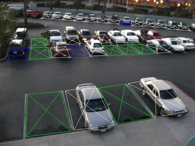
So I finally finished my color histogramming program. Since training the support vector machine is completely pointless unless the data you are training it on is accurate, I had to make sure that my 'histogrammer' was 100% bug free. Here are some of the test images I used to debug the program:

Currently, the program works by reading in the log file which contains a list of coordinate-image lines to extract the pixels from a particular region of an image. For each line in the log file the program does the following:

1. Compute the extraction region in the image.
   
2. Convert the image from RGB to L*a*b*.
3. Create 2 32-bin histograms, one for the 'a' channel and one for the 'b' channel (we discard the 'L' channel as it does not add much useful information in this case).
4. Compute the histograms.
5. Write out each histogram, bin by bin, to the resulting text file along with a 0 or a 1 to indicate if the region was a positive or negative training example.

With a log file of exactly 800 training regions, the program only took a couple of minutes to finish its calculations.

My next step will be to train a support vector machine on this training data. Since I'm most familiar with SVMLight, I'm probably going to start there.